4 - Uses of Partial derivatives

Prev Next

Calculus of Multivariable Functions

Section 4 Use of the Partial Derivatives

Marginal functions

For a multivariable function which is a continuously differentiable function, the first-order partial derivatives are the marginal functions, and the second-order direct partial derivatives measure the slope of the corresponding marginal functions.

For example, if the function $f(x,y)$ is a continuously differentiable function,
Marginal function with respect to $x$ is $f_{x}$.
Slope of the marginal function $f_{x}$is $f_{xx}$.
Marginal function with respect to $y$ is $f_{y}$.
Slope of the marginal function $f_{y}$ is $f_{yy}$.

Measuring the slope

Consider a multivariable function $= f(x,y)$. Suppose, for each pair of $(x,y)$, we evaluate $f(x,y)$ to obtain the same value of $z$, say $z_{0}$. If we draw the locus in the $xy$-plane of $(x,y)$ pairs for which the function has the value $z_{0}$, the corresponding curve is called the level curve of the function (See Simon and Blume, p 280). In economics frequently used level curves are indifference curves and isoquants. If we draw the level curve of $z = f(x,y) = z_{0}$ while measuring $y$ on the vertical axis and $x$ on the horizontal axis, the slope of the level curve is $$\frac{dy}{dx} = -\frac{f_{x}}{f_{y}} = -\frac{\frac{\partial f(x,y)}{\partial x}}{\frac{\partial f(x,y)}{\partial y}}$$ Example:
Consider the function $f(x,y) = 2x + 3y$. The slope of the level curve is $\frac{dy}{dx} = -\frac{f_{x}}{f_{y}} = -\frac{2}{3}$.
For a Cobb-Douglas function $f(x,y) = x^{\alpha }y^{\beta }$, the slope of the level curve is $-\frac{f_{x}}{f_{y}} = -\frac{\alpha y}{\beta x}$.

Marginal rate of substitution (MRS)

Consider a multivariable function $f(x,y)$ which is a continuously differentiable function. For such functions, partial derivatives can be used to measure the rate of change of the function with respect to $x$ divided by the rate of change of the function with respect to $y$, which is $\frac{f_{x}}{f_{y}}$. If there exists level curves for the function $f(x,y)$, the ratio $\frac{f_{x}}{f_{y}}$ is called the marginal rate of substitution.

For example, if a function is $f(x,y) = 2x + 3y$, then $\frac{f_{x}}{f_{y}} = \frac{2}{3}$ is the marginal rate of substitution between $x$ and $y$ for its corresponding level curves.
For a Cobb-Douglas function $f(x,y) = x^{\alpha }y^{\beta }$, the marginal rate of substitution between $x$ and $y$ for its corresponding level curves is $\frac{f_{x}}{f_{y}} = \frac{\alpha y}{\beta x}$.
If the Cobb-Douglas function is $f(x,y) = x^{0.5}y^{0.5}$, the level curve corresponds to the point $(4,16)$ is $x^{0.5}y^{0.5} = (4)^{0.5}(16)^{0.5} = 8$. The marginal rate of substitution between $x$ and $y$ at $(4,16)$ is $\frac{f_{x}}{f_{y}} = \frac{\alpha y}{\beta x} = \frac{0.5(16)}{0.5(4)} = 4$.

Finding the extreme values

A point in a multivariable function may be an extreme point if it meets the following necessary conditions:

All first partial derivatives of the function, evaluated at that point, must be equal to zero simultaneously (that means the function is neither increasing nor decreasing with respect to any of the independent variables at that point.)

For example, consider a function $f(x,y)$ which is a continuously differentiable function. At the extreme points (local max or local min, if any), each first-order partial derivative must be simultaneously zero: $$f_{x} = 0$$ $$f_{y} = 0$$ By solving these simultaneous equations, we get the pair $(x,y)$, which is called the critical value of the function. If there is an extreme value of the function, the critical value will determine the extreme value.

Note: The existence of the critical point is a necessary condition to get the extreme value if any exists. However, the existence of a critical point is not sufficient enough to tell that there exists an extreme value at that critical point and that the extreme value is a local max or a local min. To check the sufficient conditions, that is to check whether the function is at an extreme point at the critical point, we need the second-order conditions for the optimization, which we will not discuss in this chapter. To study the second-order conditions for optimization of functions of several variables, please use suggested readings when required.

Some Examples

Example 1: Find the marginal functions: $$f(x,y) = 4x^{2} + 2xy + 2y^{2}$$

First-order partial derivatives measure the corresponding marginal functions. $$f_{x} = 8x + 2y$$ $$f_{y} = 2x + 4y$$

Example 2: Find the marginal functions when $x = 2, \; \bar{y} = 3$ $$f(x,y) = 4x^{2} + 2xy + 2y^{2}$$

$$f_{x} = 8x + 2y = 8(2) + 2(3) = 16 + 6 = 22$$ Here, $f_{y} = 0$, as long as the value of $y$ is fixed.

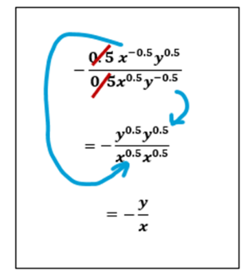
Example 3: Consider the multivariable function $f(x,y) = x^{0.5}y^{0.5}$. For its corresponding level curves, find $\frac{dy}{dx} = -\frac{f_{x}}{f_{y}}$ and the marginal rate of substitution $MRS_{x,y}$.

$$\frac{dy}{dx} = -\frac{f_{x}}{f_{y}} = -\frac{0.5x^{-0.5}y^{0.5}}{0.5x^{0.5}y^{-0.5}} = -\frac{y^{0.5}y^{0.5}}{x^{0.5}x^{0.5}} = -\frac{y}{x}$$ (Rules of exponents are important here for the simplification.) $$MRS_{x,y} = \frac{f_{x}}{f_{y}} = \frac{y}{x}$$

Example 4: Suppose the multivariable function is $f(x,y) = x^{0.6}y^{0.3}$. Find the slope of the level curve $\frac{dy}{dx} = -\frac{f_{x}}{f_{y}}$ and the marginal rate of substitution $(MRS_{x,y})$.

$$\frac{dy}{dx} = -\frac{f_{x}}{f_{y}} = -\frac{0.6x^{-0.4}y^{0.3}}{0.3x^{0.6}y^{-0.7}} = -2\frac{y^{0.3}y^{0.7}}{x^{0.6}x^{0.4}} = -\frac{2y}{x}$$ $$MRS_{x,y} = \frac{f_{x}}{f_{y}} = \frac{2y}{x}$$

Example 5: Suppose the multivariable function is $f(x,y) = x^{0.6}y^{0.4}$. Find the slope of the level curve $\frac{dy}{dx} = -\frac{f_{x}}{f_{y}}$ and the marginal rate of substitution $(MRS_{x,y})$.

(If you understand the steps and the calculation process, why need to repeat all the steps?) $$Slope = -\frac{f_{x}}{f_{y}} = -\frac{3y}{2x}$$ $$MRS_{x,y} = \frac{3y}{2x}$$

Example 6: Find the critical points, if any exists: $$z = 20y - 2x^{2} - 4xy - y^{2} + 30x$$

A necessary condition for the existence of a critical point is that all first-order partial derivatives must be simultaneously $0$: $$z_{x} = -4x - 4y + 30 = 0 \qquad\qquad \text{(1)}$$ $$z_{y} = -4x - 2y + 20 = 0 \qquad\qquad \text{(2)}$$ From these two simultaneous equations we can eliminate $x$ by deducting Equation (2) from Equation (1) to get: $$-2y = -10$$ $$y = 5$$ Substitute y=5 in either (1) or (2) to get $$x = 2.5$$ Here the critical point is $(2.5,5)$. If there exists an extreme point (local max or min), that will correspond to this critical point. To check if the function is at an extreme point at the critical point, we need to check the second-order conditions for optimization. A list of books is attached at the end of this chapter which can be used to learn more about the second-order conditions.

Cobb-Douglas Function

This chapter mainly discusses the calculus of multivariable functions using the Cobb-Douglas form of functions. The standard form of a Cobb-Douglas function with two unknowns is: $$f(x,y) = Ax^{\alpha}y^{\beta}$$ Where, $A$ shows the technological parameter which is a constant and greater than $0$, and $\alpha $ and $\beta $ are the exponents which are also greater than $0$.
The exponent $\alpha $ shows the $x$-elasticity of the function $f(x,y)$, or simply the responsiveness of the function to a change in the variable $x$. For example, if $\alpha = 0.5$, a $1$% increase in $x$ would lead to an approximately $0.5$% increase in $f(x,y)$ given that $y$ remains constant. The exponent $\beta $ shows the $y$-elasticity of the function $f(x,y)$.
Cobb-Douglas functions have many important properties. Most importantly, if the utility functions and the production functions take the form of Cobb-Douglas functions, then the corresponding level curves showing the indifference curves and isoquants are downward sloping, non-linear, and convex to the origin with slope $\frac{dy}{dx} = -\frac{\alpha y}{\beta x}$ and marginal rate of substitution $MRS_{x,y} = \frac{\alpha y}{\beta x}$. We discuss more about Cobb-Douglas functions in the subsequent sections. But we recommend reading more about the Cobb-Douglas functions and their properties.