Section 6
Use of Partial Derivatives in Economics; Some Examples
Marginal functions
Given that the utility function \(u = f(x,y)\) is a differentiable function and a function of two goods, \(x\) and \(y\):
Marginal utility of \(x\), \(MU_{x}\), is the first order partial derivative with respect to \(x\)
And the marginal utility of \(y\), \(MU_{y}\), is the first order partial derivative with respect to \(y\)
Similarly, if the production function is a function of capital \((K)\) and labor \((L)\), \(Q = f(K,L)\), the marginal product of capital, \(MP_{K}\), is measured by taking the first order partial derivative with respect to \(K\) and the marginal product of labor, \(MP_{L}\), is measured by taking the first-order partial derivative with respect to \(L\).
Example 1: From the following production function, find the marginal product of capital, \(MP_{K}\) and the marginal product of labor, \(MP_{L}\). $$Q = 10K^{0.5}L^{0.5}$$
Marginal product of capital, $$MP_{K} = \frac{\partial Q}{\partial K}$$ $$\qquad\quad = (10)(0.5)K^{0.5 - 1}L^{0.5}$$ $$\qquad\quad = 5K^{-0.5}L^{0.5}$$ Marginal product of labor, $$MP_{L} = \frac{\partial Q}{\partial L} = 5K^{0.5}L^{0.5 - 1} = 5K^{0.5}L^{-0.5}$$
Example 2: From the following utility function, find the marginal utility of \(x\), \(MU_{x}\), and the marginal utility of \(y\), \(MU_{y}\). $$u = x^{0.4}y^{0.6}$$
Marginal utility of \(x\), $$MU_{x} = \frac{\partial u}{\partial x} \qquad\qquad\qquad\qquad\qquad\qquad\;$$ $$= 0.4x^{0.4 - 1}y^{0.6} = 0.4x^{-0.6}y^{0.6}$$ Marginal utility of \(y\), $$MU_{y} = \frac{\partial u}{\partial y} = 0.6x^{0.4}y^{0.6 - 1} = 0.6x^{0.4}y^{-0.4}$$
Measuring the slopes of indifference curves and isoquants
An indifference curve connects consumption baskets that yield the same level of satisfaction for the consumer. Suppose a consumer consumes two goods, \(x\) and \(y\). An indifference curve shows a set of different combinations of \((x,y)\) for which the consumer gets equal satisfaction, say for example, \(k\): $$u(x,y) = k$$ Where, \(k\) is a constant.
A typical indifference curve is drawn below.
Figure 1
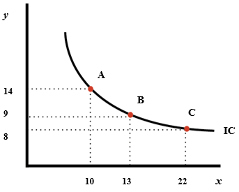
Suppose the consumer moves from \(A\) to \(B\) in the same indifference curve. This movement leads to a change in \(x\), which is \(dx\), and a change in \(y\), which is \(dy\). The change in the utility due to the change in \(x\) is, \(MU_{x}dx\). The change in the utility due to the change in \(y\) is, \(MU_{y}dy\). However, at the end, there is no change in the total utility as the consumer remains on the same indifference curve. Hence, we can write that, on the same indifference curve: $$(\text{marginal utility of } x) \times (\text{change in } x) + (\text{marginal utility of } y) \times (\text{change in } y) = 0$$ $$MU_{x}dx + MU_{y}dy = 0$$ $$\qquad\qquad\qquad\qquad\; MU_{y}dy = -MU_{x}dx$$ $$\qquad\qquad\qquad\qquad\quad\; \frac{dy}{dx} = -\frac{MU_{x}}{MU_{y}}$$ Here \(MU_{x} = \frac{\partial u(x,y)}{\partial x}\) and \(MU_{y} = \frac{\partial u(x,y)}{\partial y}\) And \(\frac{dy}{dx} = -\frac{MU_{x}}{MU_{y}}\) is the slope of the indifference curve.
Similarly, we can find the slope of an isoquant, a curve showing different combinations of factors of production, capital \((K)\) and labor \((L)\) that yield the same level of production \((Q)\).
If the isoquant is \(Q(K,L) = k\), where \(k\) is a constant,
Its slope is: $$\frac{dK}{dL} = -\frac{MP_{L}}{MP_{K}}$$ By this time, you should be familiar with the terms \(MU\) (marginal utility, not miss you!) and \(MP\) (marginal product).
Example 3: Suppose the equation of an indifference curve is \(u(x,y) = xy = 10\). Calculate the slope of the indifference curve.
$$\frac{dy}{dx} = -\frac{MU_{x}}{MU_{y}}$$ $$= -\frac{\left ( \frac{\partial (xy)}{\partial x} \right )}{\left ( \frac{\partial (xy)}{\partial y} \right )}$$ $$= -\frac{y}{x}$$
Example 4: Suppose the equation of an isoquant is \(Q(K,L) = K^{0.5}L^{0.5} = 200\). Calculate the slope of the isoquant.
$$\frac{dK}{dL} = -\frac{MP_{L}}{MP_{K}}$$ $$= -\frac{\left ( \frac{\partial (K^{0.5}L^{0.5})}{\partial L} \right )}{\left ( \frac{\partial (K^{0.5}L^{0.5})}{\partial K} \right )}$$ $$= -\frac{K}{L}$$
Marginal rate of substitution (MRS) and marginal rate of technical substitution (MRTS)
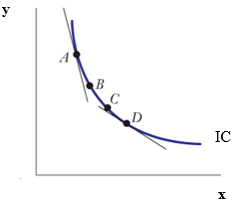
The marginal rate of substitution measures a consumer’s willingness to substitute one good for another while remaining on the same indifference curve. Generally, the \(MRS_{x,y}\) at a point is the negative of the slope of the indifference curve at that point. For example, in the following graph, the slope of the indifference curve at point \(A\) is \(-5\), implying that the \(MRS_{x,y}\) at point \(A\) is \(5\). This says that at Point \(A\), the consumer is ready to sacrifice \(5\) units of \(y\) for only \(1\) unit of \(x\) holding the utility constant. The \(MRS\) is not same everywhere along a typical downward sloping, non-linear, convex indifference curve. For example, at point \(D\) of the same indifference curve below, the slope of the indifference curve is \(-2\), implying that the \(MRS_{x,y}\) at point \(D\) is \(2\). The consumer is willing to sacrifice only \(2\) units of \(y\) to get \(1\) unit of \(x\). This is because at point \(D\), the consumer already has more \(x\) compared to the bundle at point \(A\) causing a decrease of his marginal utility from \(x\).
Figure 2
Similarly, we measure the marginal rate of technical substitution, \(MRTS_{L,K}\), by first deriving the slope and then by taking the absolute value of the slope. The value of \(MRTS_{L,K} = 5\) means, by substituting \(5\) units of \(K\) for \(1\) unit of \(L\), it is still possible to produce the same level of output around that point.
Please remember the words typical, general, etc. because for the special cases these characteristics may not hold. If two goods are perfect substitutes, for example, tea and coffee, then the \(MRS\) is constant along the indifference curve. And if two goods are perfect complements, for example, left shoe and right shoe, there exist no substitution between the goods. In the entire chapter, we discuss the general/typical cases where the indifference curves and isoquants are non-linear, downward sloping, convex to the origin and follow other usual properties of the Cobb-Douglas function. We also overlook any discussion about bad, neutral goods, and corner solutions, etc. in this chapter.
Example 5: Suppose the equation of an indifference curve is \(u(x,y) = xy = k\). Calculate the \(MRS_{x,y}\) at the following points: A (2,8) and B (8,2).
$$\frac{dy}{dx} = -\frac{MU_{x}}{MU_{y}}$$ $$= -\frac{\left ( \frac{\partial (xy)}{\partial x} \right )}{\left ( \frac{\partial (xy)}{\partial y} \right )}$$ $$= -\frac{y}{x}$$ $$MRS_{x,y}(2,8) = \frac{y}{x} = \frac{8}{2} = 4$$ $$MRS_{x,y}(8,2) = \frac{y}{x} = \frac{2}{8} = 0.25$$
Example 6: Suppose the equation of an isoquant is \(Q(K,L) = K^{0.5}L^{0.5} = k\). Calculate the \(MRTS_{L,K}\) when \(L = 4\) and \(K = 4\).
$$MRTS_{L,K} = \frac{MP_{L}}{MP_{K}}$$ $$= \frac{\left ( \frac{\partial (K^{0.5}L^{0.5})}{\partial L} \right )}{\left ( \frac{\partial (K^{0.5}L^{0.5})}{\partial K} \right )}$$ $$= \frac{K}{L}$$ $$MRTS(4,4) = \frac{4}{4} = 1$$

UWO Economics Math Resources by Mohammed Iftekher Hossain is licensed under a Creative Commons Attribution-NonCommercial-ShareAlike 4.0 International License.