Section 8

Use of Multivariable Calculus in Analyzing the Producer Behavior: Some Examples

(Some knowledge about the competitive market, price determination, the difference between market and firm, cost functions, short-run and long-run in microeconomics, etc. are important to understanding this section. This section is a review of the related concepts using examples and does not explain the concepts in detail. For a detail discussion, please read recommended books, or follow the links in the important link.)

We will discuss a few examples in this section from the competitive market to illustrate how the calculus of multivariable functions are relevant in the firm’s decision making of cost and output. We will not discuss the price determination in this section as we will discuss the examples of firms operating in the competitive markets where the price is determined in the market, and it’s given for the price-taking firms. However, in the case of non-competitive markets, for example, monopoly or oligopoly, multivariable calculus is an important tool to determine the market price.

We start by relaxing the assumption that the firm uses only one input to produce its output. However, for simplicity, we assume that the firm uses only two inputs, capital \((K)\) and labor \((L)\). Factors of production are not free in the market, even if you are the owner of the firm, your own labor is not free of cost, there is an opportunity cost. Suppose that the price of capital is \(P_{K} = r\) and the price of labor is \(P_{L} = w\). And suppose that we are considering the long run of the firm where there is no fixed input and therefore no fixed cost. Hence, the cost of the firm while using \(K\) and \(L\) is $$C = rK + wL$$ The higher is the production, the more capital and labor are required, and the higher is the cost. How much capital and labor are required depend on the production function. Suppose, the production function is a function of two factors of production, \(K\) and \(L\), and can be written as \(Q(K,L)\) or \(f(K,L)\). This is the general form of the production function and a specific form of the production function, for example, is: \(Q = 10K^{0.7}L^{0.3}\). The production function shows the amount of output that can be produced if \(K\) and \(L\) are efficiently used. If you understand these concepts and multivariable calculus, you can play with these functions to find the minimum cost, maximum output, maximum profit, homogeneity, return to scale, output elasticity etc. If you continue to study economics, you will learn these techniques over time. In this section, we will focus on only to discuss the example from the cost minimization of a competitive firm using the techniques of multivariable calculus.

Suppose a competitive firm uses capital \((K)\) and labor \((L)\) to produce a good, say \(x\) and based on the technology and the production process, suppose the production function takes the following form: $$Q(K,L) = 5K^{0.5}L^{0.5}$$

Suppose in our example the market prices of K and L are: $$P_{K} = r = 10$$ $$P_{L} = w = 10$$ The firm faces the cost function: $$C = rK + wL = 10K + 10L$$ Suppose the firm has a target production of, say \(80\) units. So, this firm faces the following constraint: $$Q(K,L) = \color{red}{2K^{0.5}L^{0.5} = 80}$$ Here the decision problem of the firm is to minimize the cost of production subject to the production constraint: $$\text{min } rK + wL$$ $$\text{Subject to } \color{red}{5K^{0.5}L^{0.5} = 80}$$ Many producers in the real-world face similar problems. Many of them are not an economics graduate. They may not be aware of multivariable calculus or economic concepts like the Cobb-Douglas etc. However, many of them are still producing the output using factors of production as efficient as possible.
Let us apply the constrained optimization tools:

Marginal product:

To take the decision to minimize cost, the concept about the marginal products are essential. Here we are considering two factors of production, \(K\) and \(L\). We can calculate the marginal product of capital \((MP_{K})\) and the marginal product of labor \((MP_{L})\) using the techniques of partial differentiation: $$MP_{K} = \frac{\partial f(K,L)}{\partial K}$$ $$MP_{L} = \frac{\partial f(K,L)}{\partial L}$$ For the given firm the marginal products are: $$\color{red}{MP_{K}} = \frac{\partial }{\partial K}5K^{0.5}L^{0.5} = 5(0.5)K^{(0.5 - 1)}L^{0.5} = 0.25K^{-0.5}L^{0.5} = 0.25\color{red}{\frac{L^{0.5}}{K^{0.5}}}$$ $$\color{red}{MP_{L}} = \frac{\partial }{\partial L}5K^{0.5}L^{0.5} = 5(0.5)K^{0.5}L^{(0.5 - 1)} = 0.25K^{0.5}L^{-0.5} = 0.25\color{red}{\frac{K^{0.5}}{L^{0.5}}}$$

Isoquant: slope and marginal rate of technical substitution (MRTS)

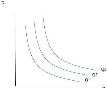
Though we mentioned it earlier, it’s worth mention here again that an isoquant curve shows the efficient combinations of \(K\) and \(L\) that produce the same level of output. We are focusing on the examples where the production function (and the corresponding isoquant) takes the form of Cobb-Douglas function. Cobb-Douglas isoquants have the following properties: downward-sloping, convex (concave up) to the origin, cannot intersect each other and the higher the isoquant the higher is the level of production (see Figure 1).

The slope of the isoquant is $$\frac{dK}{dL} = -\frac{MP_{L}}{MP_{K}}$$ And by this time, you are familiar with the concepts of the slope, \(MP_{L}, MP_{K}\). The slope is negative.

The marginal rate of technical substitution \(MRTS_{L,K}\) is the negative of the slope of the isoquant. These concepts are similar like the concepts we studied before in consumer’s behavior.

For the given competitive firm, the slope of the isoquant is: $$\frac{dK}{dL} = -\frac{MP_{L}}{MP_{K}} = -\frac{0.25K^{0.5}L^{-0.5}}{0.25K^{-0.5}L^{0.5}} = -\frac{K^{0.5}K^{0.5}}{L^{0.5}L^{0.5}} = -\frac{K}{L}$$ And $$\color{red}{MRTS_{L,K}} = -(-\frac{K}{L}) = \frac{K}{L}$$ If the firm uses \(64\) units of capital \((K)\), and \(4\) units of labor \((L)\), the firm can produce \(80\) units using its production function \(f(K,L) = 5K^{0.5}L^{0.5}\). If the firm uses \(K = 64\), and \(L = 4\), the \(MRTS_{L,K} = \frac{64}{4} = 16\). That means at this point the firm can give up \(16\) units of capital for \(1\) more unit of labor to produce the same level of output.

The question is how much capital and labor the firm should use to produce \(80\) units of the output by minimizing cost? \(K = 64\), and \(L = 4\)? \(K = 4\), and \(L = 64\)? any other combinations? The concepts of slope and MRTS help the firm to take the best decision about hiring the inputs.

Cost-minimizing input bundles

The firm can use the techniques of Lagrange function to solve his problem and to choose the input combination which will minimize the cost of production but at the same time will ensure enough \(K\) and \(L\) to produce \(80\) units.

It can also be solved using the geometric approach. As we are considering the Cobb-Douglas production function for which the optimal solution lies on an interior point where the slope of the objective function is tangent to the slope of the constraint function, we can apply the geometric approach to solve this problem.

Step 1 & 2: As the production function takes the form of Cobb-Douglas functions, the optimal input bundle is there where the slope of the isoquant equals the factor price ratio.

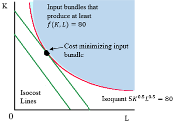
  Slope of the isoquant \(\frac{dK}{dL} = -\frac{K}{L}\) $$MRTS = -(\text{slope of the isoquant}) = K/L$$   Factor price ratio \(\frac{P_{L}}{P_{K}} = \frac{w}{r} = \frac{10}{10} = 1\)

Step 3: $$MRTS = \text{Price ratio}$$ $$\frac{K}{L} = 1$$ $$K = L$$   The firm will use the same amount of capital and labor to produce the desired output.

Step 4
  Use the relation \(K = L\) in the constraint function to solve for the optimal input bundle: $$f(K,L) = 5K^{0.5}L^{0.5} = 80$$ $$5K^{0.5}(K^{0.5}) = 80$$ $$K = \frac{80}{5} = 16$$ $$L = 16$$   Cost minimizing input bundle for the firm is \((K = 16, L = 16\)).

Concluding remarks:

Once you are familiar with the basic techniques discussed in this chapter, you will be able to play with these instruments. You will find it easier to understand the concepts related to the comparative static properties, deriving the cost functions and input demand functions, applying the techniques of Lagrange functions, profit maximization, etc. You will also have more confidence in solving the problems involving perfect substitutes, perfect complements, quasi-linear functions any many more. If you study mathematical economics, you will continue to apply the similar techniques, and you will also learn how to confirm that the cost is minimum, the utility is maximum, etc. using the second-order sufficient conditions. So far, this chapter makes us familiar with Cobb and Douglas, but knowing about Young, Hesse and many others are also important. Nevertheless, first, develop your understanding and confidence in applying the basic techniques of calculus using the typical examples that are discussed here.