8 - Producer behaviour

Prev Next

Derivatives and their uses

Section 8 Uses of the derivatives in explaining producer behaviour

In this section, we briefly discuss the behaviour of a competitive firm using the concepts of derivatives. The firm operates in the competitive market, where there are many other firms produce and sell the homogeneous product $x$, entry and exit of firms in the market are free, and all the firms and the consumers in the market have perfect information about the quality and price of the product.

Revenue:

For the competitive firm, the price of the product is given. Price $(P)$ is determined in the market, at the intersection of the market demand curve and the market supply curve. The firm cannot influence the price at all, because it is in the competitive market, and compared to the entire market the firm is very small. Therefore, the firm is a price taker and takes the price as given. Good thing is, the firm can sell all its output at the given price.

Firm's revenue function

$R(x) = P \cdot x$

Marginal revenue function:

$MR = \frac{dR(x)}{dx} = \frac{d}{dx}Px = P$

For a competitive firm, market price, $P$, represents the marginal revenue function. While the total revenue function $TR = Px$ is a linear, upward-sloping line from the origin, the marginal revenue function $MR = P$ is a horizontal line starting from $P$.

Cost:

Suppose that the firm’s cost is $C(x)$ if it produces and sells $x$ units in the market. Suppose that the firm operates in the short-run; a portion of its total cost is the fixed cost which is associated with the fixed factors. The cost function can be written as: $$C(x) = VC(x) + F$$ Where $VC(x)$ represent the variable cost and $F$ is the fixed cost. For example, if the cost function is $$\qquad\quad C(x) = x^{3} - 6x^{2} + 15x + 25$$ $$VC(x) = x^{3} - 6x^{2} + 15x$$ $$F(x) = 25 \qquad\qquad\quad\;\;$$ If the cost function of the firm is continuous and differentiable, its derivative is called the marginal cost: $$\frac{dC(x)}{dx} = MC(x)$$ Suppose the firm faces a typical cost curve with the following properties:

The cost curve is an increasing function: ${C}'(x) > 0$
Initially, the cost increases at a decreasing rate; the cost curve is initially concave. Suppose the cost curve is concave when $0 \leq x < a$. In this range ${C}''(x) < 0$ implying that the cost curve is concave.
At a point of the cost curve, concavity changes, and suppose that the point where the concavity changes, an inflection point, is $a$. At this point the second-order derivative is zero: ${C}''(a) = 0$.
After the inflection point, total cost increases at an increasing rate; the cost function becomes convex. So, for $x > a, {C}''(x) > 0$.
As the cost function is always increasing very reasonably-the higher the production, the higher is the requirement for the inputs, the higher is the cost- ${C}'(x) \neq 0$.

As the firm faces the typical total cost function, $C(x)$, its marginal cost curve, $MC(x)$, is U-shaped (not your shape though).

In part, where ${C}''(x) < 0$, total cost increases at a decreasing rate, the marginal cost is decreasing.
At the inflection point of the total cost function where ${C}'(x) > 0$ and ${C}''(x) = 0$ marginal cost is the lowest.
When the marginal cost is the lowest, it is still greater than zero, as the additional cost to produce an additional unit cannot be zero or negative. Mathematically, $MC(x) = {C}'(x) > 0$
In any suggested reading, you should see the discussion about the relationship between the marginal cost, $MC(x)$ and the average cost, $AC(x)$. If the total cost curve $C(x)$ is initially concave and then convex, then both the $MC(x)$ and $AC(x)$ are U-Shaped and the $MC(x)$ cuts the $AC(x)$ at its lowest point.

Firm's optimization problem:

The competitive firm faces the following optimization problem:
Optimize (or maximize), $$\pi(x) = R(x) - C(x)$$ The first-order condition for the profit maximization is $$\qquad\qquad {\pi}'(x) = {R}'(x) - {C}'(x) = 0$$ $$MR(x) - MC(x) = 0 \qquad\qquad$$ $$\qquad\qquad MR(x) = MC(x)$$ For the competitive firm: $MR(x) = P$
Therefore, the first-order necessary condition for the profit maximization can be written as: $$P = MC(x)$$ The firm will produce $x$ up to the level where $P = MC(x)$. As long as, $P > MC(x)$, the firm will increase its production. If $P < MC(x)$, the firm will cut the production of those units for which $P < MC(x)$. The firm, to maximize profit, will settle its output where $P = MC(x)$.

Necessary vs. sufficient conditions

If the $MC(x)$ curve is U-shaped as we discussed in the cost-section, there are two points where $P = MC(x)$. Firm’s profit is not at a maximum at both these points.
The profit is at a maximum at the point which satisfies the second-order sufficient condition for the maximization. The second-order sufficient condition is that the extreme point to be a maximum, the function must be concave at that point. Mathematically, the second-order condition is: ${\pi}''(x) < 0$.
In the context of the competitive firm, the second-order sufficient condition is: $${\pi}''(x) = {R}''(x) - {C}''(x) < 0$$ $${C}''(x) > {R}''(x)$$ ${R}'(x)$ is the marginal revenue, and ${R}''(x)$ is the slope of the marginal revenue function. As for the competitive firm, ${R}'(x) = P$ is a constant function, the slope of the marginal revenue function is zero.
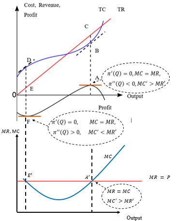
The second-order derivative of the cost function, ${C}''(x)$, is the slope of the marginal cost function. The marginal cost function, which is U-shaped, cuts the marginal revenue function of the competitive firm twice. At one intersection point, the slope of the marginal cost function is negative. When the marginal cost curve is negatively sloped, the second-order sufficient condition ${C}''(x) > {R}''(x)$ is not met. The intersection point which lies on the upward sloping part of the $MC$ curve satisfies the second-order sufficient condition as in that intersection point, the slope of the marginal cost function is greater than $0$ whereas the slope of the marginal revenue function is $0$. Figure 15 presents the cost, revenue, and profit functions of a competitive firm.

Figure 15

To sum up:
The optimization problem of the competitive firm is:

Max $\pi = Px - C(x)$

First-order necessary condition is: $${\pi}'(x) = \frac{d\pi}{dx} = MR - MC = P - MC = 0$$ Second-order sufficient condition is:

${\pi}''(x) = M{R}'(x) - M{C}'(x) < 0$
Slope of the $MC(x)$ $>$ Slope of $MR(x)$
Slope of the $MC(x) > 0 \qquad\qquad$

(To read more about the input and output decision of a competitive firm, please click the important link in the resources.)