7 - Economics uses

Prev Next

Derivatives and their uses

Section 7 Uses of the derivatives in economics

Marginal functions

Marginal function in economics is defined as the change in total function due to a one unit change in the independent variable. If the total function is a continuous function and differentiable, by differentiating the total function with respect to the corresponding independent variable, the marginal function can be obtained.

Marginal cost is the change in total cost incurred from the production of an additional unit. Given that the total cost function $TC = TC(q)$ is a continuous and differentiable function, the first-order differentiation of the total cost function is the corresponding marginal cost function:

If $TR = TR(q)$

$\frac{dTC}{dq} = MC(q)$

Marginal revenue is the change in total revenue brought about by selling one extra unit of output. Given that the total revenue function $TR = TR(q)$ is a continuous and differentiable function, the first-order differentiation of the total revenue function is the corresponding marginal revenue function:

If $TR = TR(q)$

$\frac{dTR}{dq} = MR(q)$

If the total product is a function of labor (L), $TP = TP(L)$, the marginal product of labor is $\frac{dTP}{dL}$

If $TP = TP(L)$

$\frac{dTP}{dL} = MP_{L}$

If the total utility of a consumer is a function of the quantity of a good she consumes, $TU = TU(x)$, which is a continuous and differentiable function, her marginal utility from the product is $dTU / dx$:

If $TU = TU(x)$

$\frac{dTU}{dx} = MU_{x}$

Optimizing economic functions

With the help of the derivatives, we can find the optimum points of economic functions, if any. For example, the use of derivatives is helpful to compute the level of output at which the total revenue is the highest, the profit is the highest and (or) the lowest, marginal costs and average costs are the smallest, etc. A producer who faces a continuous and differentiable profit function, $\pi = TR(x) - TC(x)$, can apply the techniques of optimization to find the optimum level of output and the corresponding profit. A consumer who has the utility function $u = f(x)$ which is continuous and differentiable, can use the optimization techniques to find the level of consumption for which her utility is the highest.

Example 1: From the following economic functions, derive the corresponding marginal functions.

Total Cost:

$TC(Q) = 10 + 2Q$

$MC(Q) = 2$

$TC(Q) = 23 + 10Q + 2Q^{2}$

$MC(Q) = 10 + 4Q$

$TC(Q) = 2Q^{3} - 3Q^{2} + 300Q + 4000$

$MC(Q) = 6Q^{2} - 6Q + 300$

$TC(x) = 2x^{3} - 3x^{2} + 300x$

$MC(x) = 6x^{2} - 6x + 300$

Total Revenue:

$TR(x) = 100Q$

$MR(x) = 100$

$TR(x) = 100Q - 4Q^{2}$

$MR(x) = 100 - 8Q$

Total Product:

$TP(L) = 90L^{2} - L^{3}$

$MP(L) = 180L - 3L^{2}$

Here $TP$ shows the total product and $MP$ is the corresponding marginal product of the labour.

Total Utility:

$TU(x) = 10x - x^{2}$

$MU(x) = 10 - 2x$

Consumption Function:

$C = 1110 + 0.75Y$

$MPC = \frac{dC}{dY} = 0.75$

Here, $C$ is the aggregate consumption, $Y$ is the aggregate income, and $MPC$ is called the marginal propensity to consume.

Example 2: Optimize the examples of following economic functions.

a) Total revenue function: $TR = 12x - x^{2}$

(see Example 2 in Section 6)

b) Marginal cost function: $MC(q) = 3q^{2} - 12q + 30$

(see Example 3 in Section 6)

c) Total cost function: $TC(q) = q^{3} - 6q^{2} + 15q + 25$

(see Example 4 in Section 6)

d) Total product function: $TP(L) = 45L^{2} - L^{3}$

(see Example 5 in Section 6)

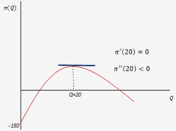
Example 3: Optimize the profit function: $$\pi (Q) = - \frac{1}{3}Q^{3} - 2Q^{2} + 480Q - 150$$ Here $\pi$ denotes the profit and $Q$ is the level of production.

First-order necessary condition for the profit maximization is that the first order derivative of the profit function is zero: $$\; {\pi}'(Q) = -Q^{2} - 4Q + 480 = 0$$ $$\;\; -Q^{2} + 20Q - 24Q + 480 = 0$$ $$-Q(Q - 20) - 24(Q - 20) = 0$$ $$\qquad\quad -(Q + 24)(Q - 20) = 0$$ $$\qquad\qquad\;\; Q = -24, \qquad Q = 20$$ As the quantity cannot be negative, $Q = -24$ is not an economic option.
$Q = 20$ holds the necessary condition for the profit maximization.
Second-order condition confirms whether the profit is maximum or minimum at $Q = 20$: $${\pi}'' = -2Q - 4 \qquad\qquad\qquad$$ $${\pi}''(20) = -40 - 4 = -44 < 0$$ The second-order condition satisfies that the profit is maximum at $Q = 20$.

Figure 13

Example 4: Explain the relationship between the total revenue $(TR)$, total cost $(TC)$ and profit $(\pi)$ functions using the following graphs.

Figure 14

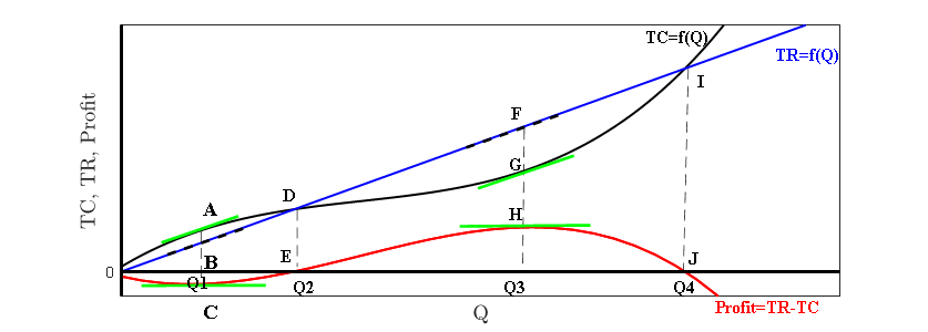
When $Q = 0$

$TC = $ Fixed cost, $TR = 0$, and $\pi = -$Fixed cost
At $Q = Q_{1}$

A Slope of the total cost function $= MC$

B Slope of the total revenue function $= MR$
$MC = MR$, as the tangents are parallel.
C Extreme point of the profit function as at $Q_{1}, MC = MR$.
However, profit at $C$ is negative as the $TC > TR$ when $Q = Q_{1}$
At $Q = Q_{2}$

D The total cost and the total revenue intersect each other, $TC = TR$

E As, $TC = TR$ at point $D$, corresponding profit is zero at point $E$
At $Q = Q_{3}$

F Slope of the total revenue function $\frac{dTR}{dQ} = MR(Q)$

G Slope of the total cost function $\frac{dTC}{dQ} = MC(Q)$
$MC = MR$ as the tangents are parallel
H $\pi$ is the highest. ${\pi}'(Q) = MR - MC = 0, {\pi}''(Q) < 0$.
At $Q = Q_{4}$

I,J $TR = TC$ and $\pi = 0$